
Sequential Decision Making With Discrete State and Action Spaces
Sequential Decision Making
Sequential decision making is a process where an agent makes a series of decisions over time, with each decision potentially affecting future decisions and outcomes. This type of decision making is crucial in dynamic environments where the agent needs to consider the long-term consequences of its actions rather than just immediate rewards.
In sequential decision making, the agent's objective is to find a policy or a strategy that specifies the action to take in each state which maximizes some notion of cumulative reward over time.
The complete code of each algorithm and method implemented in this project is available here along with all the final solutions.
Markov Decision Process (MDP)
Sequential decision making is often modeled using a Markov Decision Process (MDP), which provides a mathematical framework for modeling decision making problems where outcomes are partly random and partly under the control of the decision-maker. MDPs provide a structured way to model environments where an agent interacts with a system to achieve a specific goal. Here are the key components of an MDP:
States (S): The state space S represents all possible configurations or situations that the agent can encounter in the environment. Each state provides a snapshot of the environment at a particular time.
Actions (A): The action space A consists of all possible actions the agent can perform. Example: moving up, down, left, right, stay in current position
Transition Function (P): The transition function P(s′∣s,a) defines the probability of moving to a new state s′ given the current state s and action a.
Reward Function (R): The reward function R(s,a,s′) assigns a numerical reward to each transition, indicating the immediate benefit or cost of moving from state s to state s′ due to action a. Rewards guide the agent's behavior towards achieving the goal.
Policy (π): A policy π is a strategy that specifies the action to take in each state. It can be deterministic (always choosing the same action in a given state) or stochastic (choosing an action according to a probability distribution).
Discount Factor (γ): The discount factor γ ranges between 0 and 1 and reflects the agent’s preference for immediate rewards over future rewards. A higher discount factor means the agent values future rewards more, leading to long-term planning.
The primary objective of an MDP is to find an optimal policy π* that maximizes the expected cumulative reward over time. The cumulative reward, also known as the return, is the total amount of reward an agent expects to accumulate starting from a given state and following a particular policy. Value Iteration and Policy Iteration are commonly used to solve an MDP and find the optimal policy.
Value Iteration
Value iteration involves iteratively updating the value function V(s) for each state until it converges to the optimal value function V*(s). The value function represents the maximum expected cumulative reward an agent can achieve from a state.
The main steps of the value iteration algorithm are as follows:
- Initialization: Start with an initial value function V0(s) for all states s. This is often initialized to zero for all states.
- Value Update: Update the value of each state using the Bellman optimality equation until the value function converges. The update rule is:

#Value Iteration
Q = np.zeros(len(A))
for a in range(len(A)):
   Q[a] = R(s,a)
   for i in range(len(A)):
      if not hit_wall(s, i):
         s_next = s_next_calc(s, i)
         Q[a] += discount * Pr(s_next, s, a, alpha) * V_prev[s_next]
V[s] = np.max(Q)
delta = max(delta, abs(V[s] - V_prev[s]))
Convergence: Repeat the value update step until the value function changes by less than a small threshold for all states, indicating convergence to the optimal value function V*.
Policy Iteration
Policy iteration consists of two main steps: policy evaluation and policy improvement. The goal is to find the optimal policy π* that maximizes the expected cumulative reward.
- Initialization: Start with an arbitrary policy π0
- Policy Evaluation: Compute the value function for the current policy πk

a = policy[s]V[s] = R(s, a)for i in range(len(A)):if not hit_wall(s, i):s_next = s_next_calc(s, i)V[s] += discount * V_prev[s_next] * Pr(s_next, s, a, alpha)# convergece testdelta = max(delta, abs(V[s] - V_prev[s])) - Policy Improvement: Update the policy π' based on the current value function.

old_action = policy[s]
Q = np.zeros(len(A))
for a in range(len(A)):
   Q[a] = R(s,a)
   for i in range(len(A)):
      if not hit_wall(s, i):
         s_next = s_next_calc(s, i)
         Q[a] += discount * Pr(s_next, s, a, alpha) * V_prev[s_next]

# update policy at state s
policy[s] = np.argmax(Q)
if old_action != policy[s]: policy_stable = False
Project Overview
Now that we have covered the fundamental concepts and definitions, including a basic understanding of Markov Decision Processes (MDPs), we can move on to applying these methods to solve actual problems.
In this project, we will experiment with navigating through a maze, starting from an initial state (1,1) and reaching the goal state (24,24). All states have a reward of -1 except for the goal state, which has a reward of 0 to incentivize the agent to reach the goal. Hitting the wall will result in a reward of -10000 (can be any high negative value) to make sure the agent never chooses an action that will lead to the wall.
Furthermore, we will implement and compare value iteration and policy iteration algorithms under different conditions including the presence of noise (stochastic) and the absence of noise (deterministic). Additionally, we will analyze the effects of varying the discount factor on the algorithms' performance and computational time.
Solution in Deterministic Policy (No Noise)
In this section, we evaluate both the value iteration (VI) and policy iteration (PI) algorithms in a deterministic environment where the noise parameter (alpha) is set to 0 and the discount factor γ set to 1. This means that the agent's actions always result in the intended state transitions without any deviation (P(s′∣s,a) = 1).

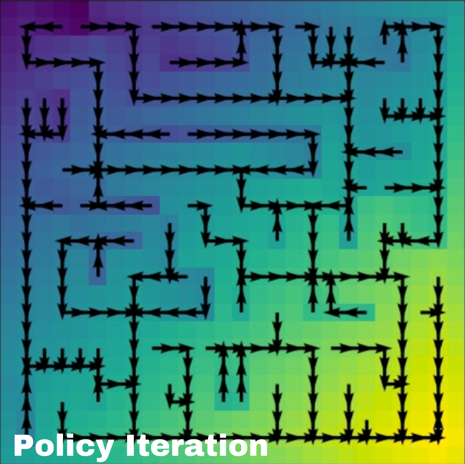
As shown in the solution images, both algorithms produced identical results, yielding the same optimal policy. The arrows in the images represent the actions chosen at each state, guiding the agent from the initial state to the goal state efficiently.
The value functions are depicted with varying shades of color. Darker colors indicate lower values, which are predominantly seen near the initial node. Lighter colors represent higher values, which are concentrated around the goal state. This gradient effect illustrates how the value increases as the agent gets closer to the goal, reflecting the expected cumulative reward.
In a deterministic environment, both algorithms converged quickly (VI in 48 iterations and PI in 42 iterations) due to the absence of noise. Each action reliably led to the intended next state, simplifying the value and policy updates. The consistency in the results of both algorithms demonstrates their effectiveness in identifying the optimal policy in a deterministic setting.
Solution in Stochastic Policy
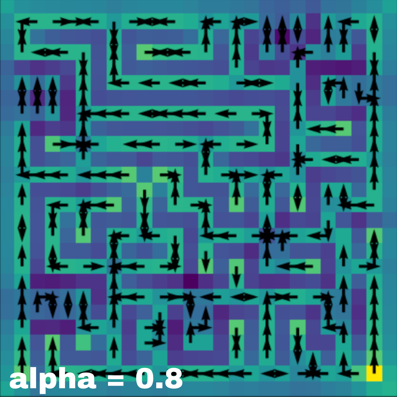
In this section, we will introduce the noise parameter (alpha) in our experiment to simulate uncertainty in the agent's actions. This means for alpha = 0.2, transition probability, P(s′∣s,a) of going up would be 0.8 for action up and the summation of P for all other actions except up would be 0.2. Both value and policy iterations are evaluated with a discount factor of 1 and noise of 0.2 and 0.8. The solutions for both the noise values using value iteration are shown below.
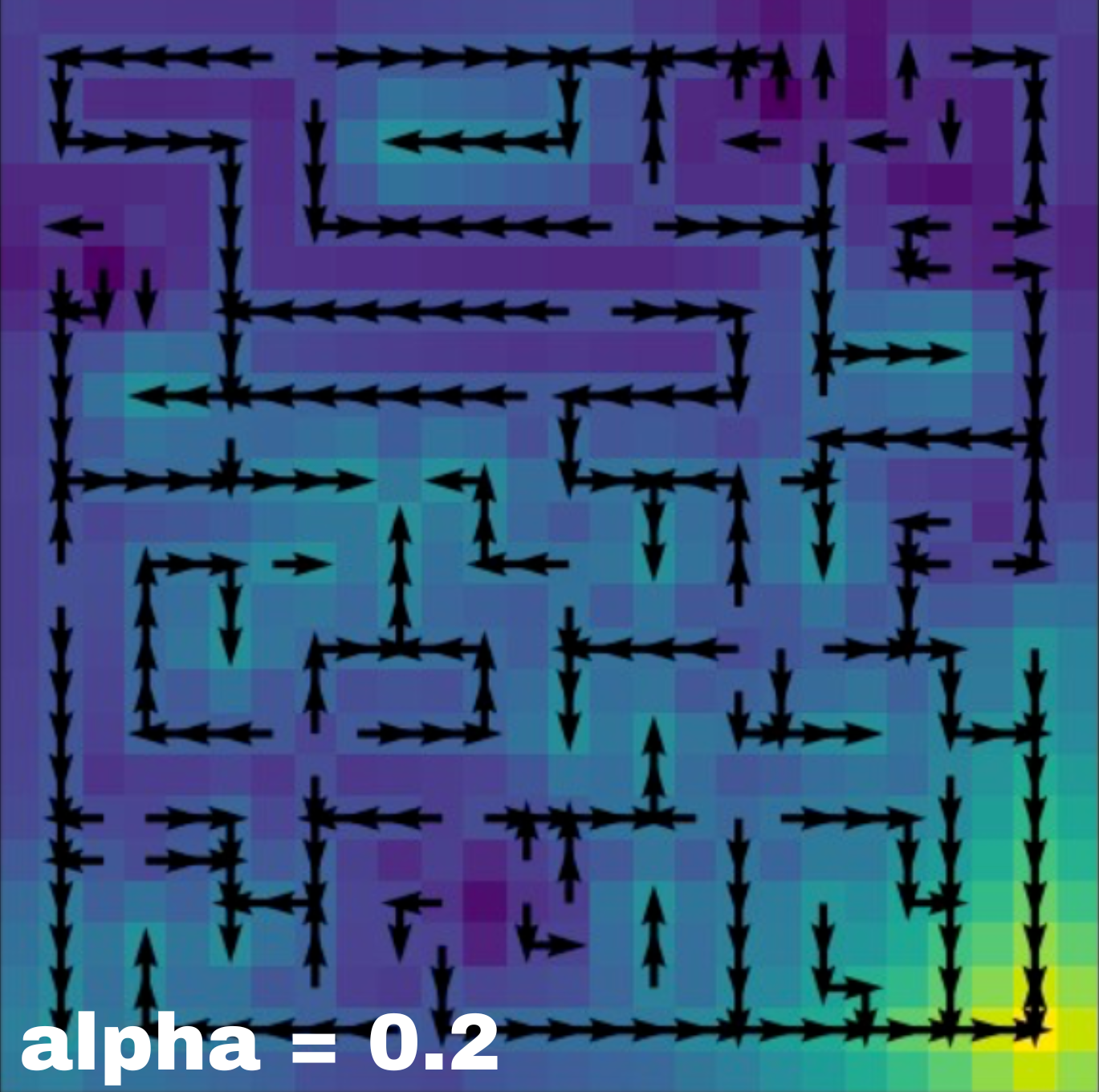
With a noise level of α=0.2, the optimal policies derived exhibit a small but noticeable impact from the zero noise solution. The arrows generally guide the agent toward the goal, but there are occasional deviations due to the stochastic nature of the transitions.
With a high noise level of α=0.8, the impact is large, significantly deviating from the optimal policy with more erratic and uncertain paths. The value function shows substantial fluctuations, leading to policies with higher uncertainty and less stability. The arrows indicate a greater degree of variability in the chosen actions, reflecting the high uncertainty in state transitions.
Impact of Discount Factor
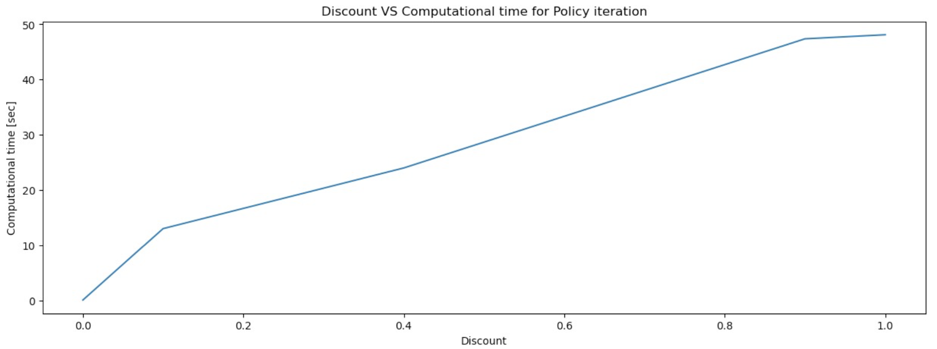
The discount factor (γ) determines how much future rewards are taken into account when evaluating the value of a state. We have chosen five different discount factors (0, 0.1, 0.3, 0.4, 0.9, 1) to explore the solution and performance of both value iteration and policy iteration algorithms.
For the simplicity of this article, I have included the images of solutions using value iteration for discount factors 0.4 and 0.9. Check the full code for all the images.
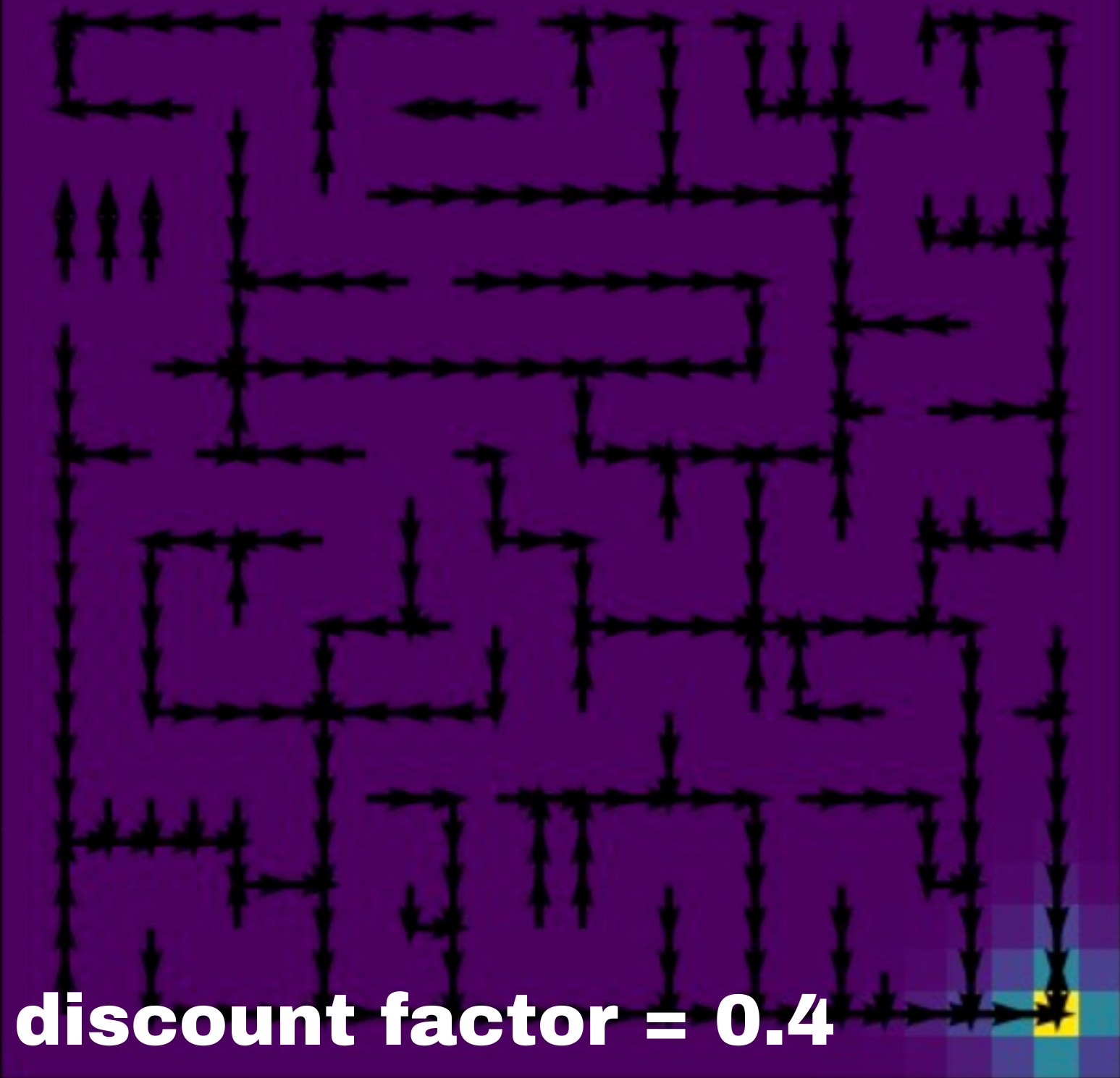
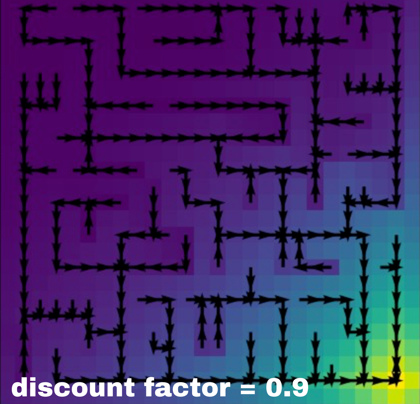
Low discount factors prioritize immediate rewards, placing little emphasis on future rewards. As a result, the policies generated are often suboptimal because they fail to consider the long-term consequences of actions. The value function is dominated by the immediate rewards, neglecting the potential benefits of future states. These algorithms tend to have shorter computational times since they require fewer iterations to evaluate immediate rewards.
High discount factors place greater emphasis on future rewards, encouraging the agent to consider long-term outcomes. This produces policies closer to the optimal solution by taking into account the cumulative rewards over the long run, leading to more strategic and effective decision-making. However, the computational time increases due to the need for more extensive calculations.
Conclusion
This article explored the intricate dynamics of sequential decision making with discrete state and action spaces using Markov Decision Processes (MDPs). Through a detailed examination of value iteration and policy iteration algorithms, we highlighted their mechanisms and applications in navigating a maze environment. Furthermore, it demonstrated the adaptability and effectiveness of these algorithms in handling various levels of stochasticity and reward prioritization.
By leveraging these powerful algorithms, we can enhance the capabilities of autonomous agents to make informed, strategic decisions in uncertain and evolving contexts, ultimately advancing the field of artificial intelligence and machine learning.
Interested in seeing the full code and experimenting with these algorithms yourself? Check out the complete code on my Github page.